Algebra Tutorials!
   
Tuesday 19th of March  
   
Home
Exponential Decay
Negative Exponents
Multiplying and Dividing Fractions 4
Evaluating Expressions Involving Fractions
The Cartesian Coordinate System
Adding and Subtracting Fractions with Like Denominators
Solving Absolute Value Inequalities
Multiplying Special Polynomials
FOIL Method
Inequalities
Solving Systems of Equations by Graphing
Graphing Compound Inequalities
Solving Quadratic Equations by Completing the Square
Addition Property of Equality
Square Roots
Adding and Subtracting Fractions
The Distance Formula
Graphing Logarithmic Functions
Fractions
Dividing Mixed Numbers
Evaluating Polynomials
Power of a Product Property of Exponents
Terminology of Algebraic Expressions
Adding and Subtracting Rational Expressions with Identical Denominators
Solving Exponential Equations
Factoring The Difference of 2 Squares
Changing Fractions to Decimals
Solving Linear Equations
Using Patterns to Multiply Two Binomials
Completing the Square
Roots of Complex Numbers
Methods for Solving Quadratic Equations
Conics in Standard Form
Solving Quadratic Equations by Using the Quadratic Formula
Simplifying Fractions 2
Exponential Notation
Exponential Growth
The Cartesian Plane
Graphing Linear Functions
The Slope of a Line
Finding Cube Roots of Large Numbers
Rotating Axes
Common Mistakes With Percents
Solving an Equation That Contains a Square Root
Rational Equations
Properties of Common Logs
Composition of Functions
Using Percent Equations
Solving Inequalities
Properties of Exponents
Graphing Quadratic Functions
Factoring a Polynomial by Finding the GCF
The Rectangular Coordinate System
Adding and Subtracting Fractions
Multiplying and Dividing Rational Expressions
Improper Fractions and Mixed Numbers
Properties of Exponents
Complex Solutions of Quadratic Equations
Solving Nonlinear Equations by Factoring
Solving Quadratic Equations by Factoring
Least Common Multiples
http:
Solving Exponential Equations
Solving Linear Equations
Multiplication Property of Equality
Multiplying Mixed Numbers
Multiplying Fractions
Reducing a Rational Expression to Lowest Terms
Literal Numbers
Factoring Trinomials
Logarithmic Functions
Adding Fractions with Unlike Denominators
Simplifying Square Roots
Adding Fractions
Equations Quadratic in Form
Dividing Rational Expressions
Slopes of Parallel Lines
Simplifying Cube Roots That Contain Variables
Functions and Graphs
Complex Numbers
Multiplying and Dividing Fractions 1
Composition of Functions
Intercepts of a Line
Powers
http:
Multiplying Two Numbers with the same Tens Digit and whose Ones Digits add up to 10
Factoring Trinomials
Exponents and Polynomials
Decimals and their Equivalent Fractions
Negative Integer Exponents
Adding and Subtracting Mixed Numbers
Solving Quadratic Equations
Theorem of Pythagoras
Equations 1
Subtracting Fractions
Solving Quadratic Equations by Graphing
Evaluating Polynomials
Slope
Angles and Degree Measure
   
Try the Free Math Solver or Scroll down to Tutorials!


Please use this form if you would like
to have this math solver on your website,
free of charge.


Graphing Linear Functions

We can graph a linear function by calculating two ordered pairs, plotting the corresponding points on a Cartesian coordinate system, and then drawing a line through the points. We typically calculate and plot a third point as a check.

To find ordered pairs, we select values for x and then calculate the corresponding values for y. Thus, the output value y depends on our choice of the input value x. For this reason, the variable y is frequently called the dependent variable and the variable x is called the independent variable.


Example 1

Make a table of at least three ordered pairs that satisfy the function f(x) = 3x - 1. Then, use your table to graph the function.

Solution

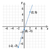
To make a table, select 3 values for x. We’ll let x = -2, 0, and 2.

Substitute the values of x into the function and simplify.

x f(x) = 3x - 1 (x, y)
-2

0

2

f(-2) = 3(-2) - 1 = -6 - 1 = -7

f(0) = 3(0) - 1 = 0 - 1 = -1

f(2) = 3(2) - 1 = 6 - 1 = 5

(-2, -7)

(0, -1)

(2, 5)


Now, plot the points (-2, -7), (0, -1), and (2, 5) and then draw a line through them.

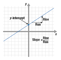
Two important characteristics of the graph of a linear function are its y-intercept and its slope.

• The y-intercept is the point where the line crosses the y-axis.

• The slope measures the steepness or tilt of the line. Slope is defined as the ratio of the rise to the run of the line. When moving from one point to another on the line, the rise is the vertical change and the run is the horizontal change.

The linear function, f(x) = Ax + B, is another way of writing the familiar slope-intercept form for the equation of a line, y = mx + b. In f(x) = Ax + B the slope of the line is given by A and the y-intercept is given by B.

f(x) = Ax + B is equivalent to y = mx + b

This means that the graphs of all linear functions are straight lines. That is why such functions are called linear.


Example 2

Graph the function:

Solution

This has the form of a linear function.
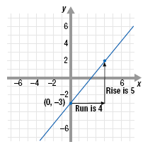
 

Thus, the slope is and the y-intercept is b = -3.

To graph the line, first plot the y-intercept; that is, plot the point (0, -3).

From this point rise in the y-direction 5 units (the numerator of the slope) and run in the x-direction 4 units (the denominator of the slope). The new location (4, 2) is a second point on the line.

Finally, connect the plotted points.

Copyrights © 2005-2024